Note
This technote describes how the sensitivity matrix, relating hexapod motion to wavefront error (modeled by Zernike Polynomials), is derived. This includes the data taking, data analysis, and relationship fitting beginning from an optical model and continuing through on-sky testing.
1 Introduction
The alignment and collimation process for the Auxiliary telescope uses the Curvature Wavefront Sensing (CWFS) alignment technique described technote tstn-015. This document describes how to determine the sensitivity matrix, which is the quantitative relationship between measured wavefront error (measured as Zernike Polynomials), relates to M2 hexapod motion. In the case of this telescope, the only correction factors being performed are the centering of the hexapod (in x and y) and the defocus (piston in z). This technote walks through the derivation of such a matrix, from the optical model estimates, then on-sky testing and verification.
One of the largest challenges of this exercise is getting the coordinate relationships correct, specifically in regards to the X/Y offset directions of the hexapod versus what they are on the detector. To add further complications is how Python uses a [Y,X] array format combined with how displays manage those images (e.g. matplotlib, firely, ds9). If one repeats this exercise they must pay strict attention to these relationships to avoid sign errors.
The format of the formula relating hexapod offsets to measured Zernike Annular (Noll) coefficients is as follows in the equation below, where the zernikes are derotated to the boresight frame. This is where the elevation and nasmyth frames are locked in rotation, meaning 90 degrees elevation is zero degrees of the instrument rotator, and similarly 60 degrees of elevation is +30 degrees of elevation.
The sensitivity matrix itself is in units of millimeters of hexapod motion per nm of measured WFE for a given Zernike polynomial. The cross-terms are best thought as scaled versions of both terms. For example, 10um of pure defocus gives 25 nm of WFE, and if 1 mm of Y-decenter results in 100 nm of coma and 50 nm of defocus, \(C_{Y}\) would be 1/100 [mm/nm] and \(D_{Z}\) would be \(0.010/50=0.0002\) [mm/um]. However, \(C_{YZ}\) indicates that there is 50 nm of defocus WFE per 100 nm of coma WFE, and then this must be scaled by the mm to nm relationship of defocus (not coma), therefore \(C_{YZ}=50/100 * D_Z = 2 * 0.0002 = 0.0004\) [mm/nm].
Important
The sensitivity matrix is for hexapod motion only. In order to build (useful) look-up tables the relationship between M1 mirror pressure versus elevation must first be derived as it strongly affects the results, primarily the defocus term. This is discussed in this technote.
2 Optical Model Output
The first approximation of the sensitivity matrix can be accomplished using the optical model of the telescope (in Zemax, Document-27702, credentials required). This was performed and it successfully measured the defocus relationship to reasonable accuracy, as well as the coma terms. This was accomplished by taking the above optical model and adding a coordinate break at the secondary mirror in order to decenter. The effect of defocusing the secondary was also added by modifying the distance between M1 and M2 and M2 and M3 by equal amounts.
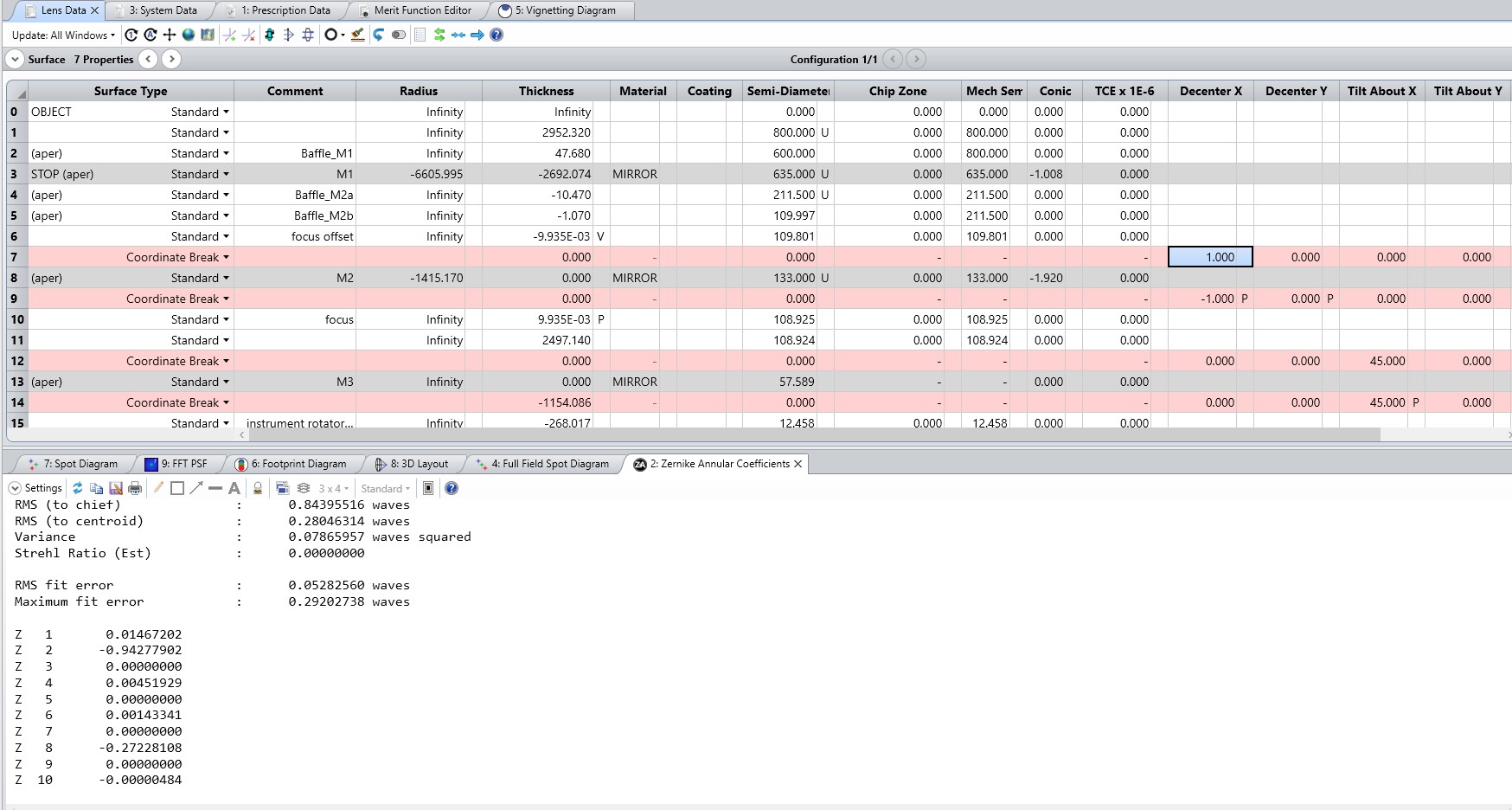
Figure 1 The sensitivity matrix can be determined from the optical model, but sign errors will most certainly result when trying to convert to image space. Elements require verification in an incremental fashion.
The terms of the sensitivity matrix in the equation above are found from offsetting the hexapod (in decenter and piston), then looking at the annular Zernike coefficients. Because the system is linear for first order terms, offsets of 1 mm were performed. The diagonal coma terms from optical model is 178 nm/mm (+1mm decenter in X is Z8=-178nm, +1 mm decenter in Y is Z7=-178nm) whereas the cross-terms (e.g \(C_{YZ}\) and \(C_{XZ}\)) are zero. Note that the X-axis here is as per Zemax conventions. The defocus term is significantly more sensitive due to the powered optics, and is estimated at 4.85 nm/um. Seeing as the magnification between the motion of the secondary mirror and the back focal distance is ~44, this is not unexpected.
Important
In the model above, it is assumed that there are no tilts in the system and that all optics are perfect. Having cross-terms are possible due to tilts in the system, but these must be measured experimentally.
3 Data Acquisition
This section discusses how to derive the experimental measurement of the sensitivity matrix. It is assumed that one starts from the matrix derived in section 2 Optical Model Output, which is purely diagonal. The general procedure of the test consists of aligning the system to the best of one’s ability at a given elevation, then stepping the hexapod in small steps and measuring the WFE. Fitting a line to this relationship gives the terms in the matrix. Performing the test successfully requires a little more thought and the following considerations should be made:
- Due to the numerous rotations in the system, it is best to choose a target that is transiting the meridian (will not greatly change in elevation) over the course of ~1.5-2 hours. Then, align the system to the best of one’s ability, which will take several iterations. Choose a target near elevation 60., as this is the mid-range of the telescope and field rotation will not be too fast
- It is strongly recommended to keep the elevation and rotator axes aligned to the extent possible (meaning the difference between rotator angle and elevation angle should be kept nearly constant. This means adjustments will be required after each pair of images.
- Perform the test later in the night, when the dome seeing has been reduced. Exposures should be ~30s long. This will require a star of magnitude ~6-8.
- Use a bandpass filter to reduce chromatic effects.
The hexapod can then be offset using relative offsets from the attcs class as shown in the following code block. Relative offsets are generally preferred as it does not require the AOS loop to be turned off.
offset = {'x':0, 'y':  0.0, 'z': 0.0}
await attcs.ataos.cmd_offset.set_start(**offset)
If you get lost or want to reset the offsets, this can be done as follows.
await attcs.ataos.cmd_resetOffset.start()
4 Data Reduction
One of the later datasets to measure the cross-terms was performed on 2020-02-18 on HD 27583. The data reduction and derivation of the matrix terms are best described from the accompanying jupyter notebook, which is found in the procedures section of the ts_notebooks repo.
The output of the notebook shows the linear fits applied to the measured Zernike coefficients, the slope of which can be input into the sensitivity matrix. The first fit shows coma as a function of offset, one would expect this to follow the optical model quite closely.
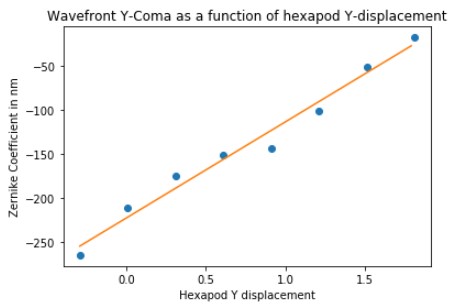
Figure 2 The slope of this fit is used in the \(C_{Y}\) term of the sensitivity matrix.
The next plot shows the derivation of the cross-term between a decenter and defocus. Due to the large magnification in the system, any mis-alignment will be heavily amplified.
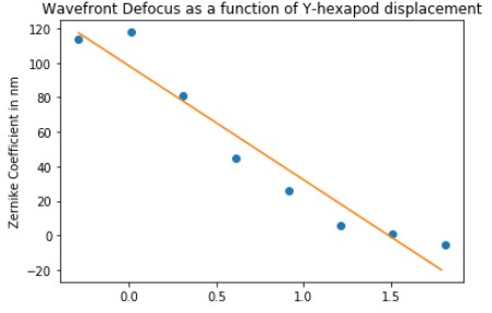
Figure 3 The slope of this fit is used in the \(C_{YZ}\) cross-term of the sensitivity matrix. Why this term is so large is a bit of a mystery.
A cross-term of 109 nm of defocus for 1 mm of lateral hexapod motion is the equivalent of ~23um of hexapod z motion. This is equivalent to having the hexapod mounted with a tilt of 1.26 degrees. Because this is ~3x larger than what one would expect from mechanical alignment therefore we suspect (but cannot confirm) that M3 is tilted and is not at exactly 45 degrees.
One can also look at the relationship between Y-hexapod motion and X-Coma. One would assume it should be largely zero.
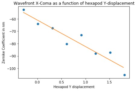
Figure 4 This could be used in the sensitivity matrix, but is omitted as it’s significantly smaller than the others and probably within the measurement errors due to turbulence.
5 Applying the Fits to the Sensitivity Matrix
The sensitivity matrix is currently only in latiss_cwfs_align.py script. In order to use another matrix, either that file must be modified, or the notebook calling it can modify it using the following code snippet:
from lsst.ts.externalscripts.auxtel.latiss_cwfs_align import LatissCWFSAlign
script = LatissCWFSAlign(index=1, remotes=False) # Change to True if taking live images
script.sensitivity_matrix = [
     [1.0 / 178.0, 0.0, 0.0],
     [0.0, -1.0 / 178.0, (109.0/178.0)/4200],
     [0.0, 0.0, -1.0 / 4200.0]
     ]
At time of writing, the summit was shutdown and we are running the scripts/notebooks on the LSP at NCSA. There are known differences in the outputs between when we ran things on the summit and what we get at NCSA. Once the summit comes back online we should be able to resolve these differences. For the moment, we recommend using the matrix above, where the diagonal terms are from the optical model and the cross terms are from the fits in the example notebook dataset.